STARKS II: Is that a polynomial?

The previous post outlined how a potentially long and complicated calculation can be represented by polynomials. Correctness of the calculation result can then be verified by checking that their values satisfy some simple identities. One issue that was avoided was how to identify if the values are indeed given by polynomials.

Bob (the prover) has performed a long and intensive calculation, and sent the result to Alice (the verifier). To be sure, Alice wants to verify the result, so requests that Bob also sends a proof of its correctness. The problem is that Alice does not have the time or computational resources to replicate the entire calculation, so it is necessary for Bob’s proof to be significantly shorter than this. So, Bob computes polynomial interpolants of the execution trace, and Alice requests their values of at a small number of random points. She checks that these values satisfy some simple algebraic identities which encode the calculation steps. If they are satisfied, then she agrees that Bob sent the correct result. However, this is assuming that Bob can be trusted. He could be sending any values selected to satisfy the identities. If we are not willing to simply trust that he has performed the original calculation correctly, why would we trust that he is really evaluating the polynomials? Alice needs a way of checking that the received values are consistent with polynomial evaluation. We will discuss how this can be done, and the solution to this problem forms a major component of STARK implementations for blockchain scaling.

Recall the setup. All polynomials are defined over a finite field F of size q = p^r for a fixed prime number p and positive integer exponent r. The case q = p is just the integers modulo p, although binary fields of size 2^r are also common. Generally, such fields are chosen to have a very large size such as 2²⁵⁶, for reasons similar to the choice of large finite fields in digital signature algorithms. It ensures that the chances of selecting one of a small number of ‘bad’ values entirely at random is negligible.

If Bob’s calculation involves some number N steps, the execution trace will be represented by polynomials of degree less than this,

(1)

The coefficients c_i are in the field F and the bound N on the degree is typically large, maybe of the order of a few million. Despite this, such polynomials are referred to as low degree. This is because the point of comparison is the size q of the field. By interpolation, every function on F can be represented by a polynomial. Most of these will have degree equal to the full size q of the field so, compared to this, N is indeed low. Such functions, consistent with a low degree polynomial, are also known as Reed–Solomon codes.

Now, Alice is able to request the values of f(x) for some randomly chosen field points x. She does not have the processing power to perform a number N operations, so is not able to evaluate the polynomial herself to check that Bob is telling the truth. She cannot even parse through all of its coefficients. The aim is to find a method for Alice to verify that the values f(x) do indeed come from a fixed polynomial of degree less than N. This is low degree testing, and needs to be done with much fewer than N operations by Alice. Something like O(logN), or a small power of this, is a reasonable level of complexity to aim for. More realistically, Alice needs to statistically check that the large majority of Bob’s values are consistent with a polynomial. This process, which is the entire focus of the current post, is known as a Fast Reed–Solomon Interactive Oracle Proof of Proximity (FRI). See the 2017 paper by Eli Ben-Sasson, Iddo Bentov, Ynon Horesh, and Michael Riabzev, for a detailed description of a specific algorithm.

---

Bob’s Commitment

The prover, Bob, needs to commit to a particular function f up-front, which Alice wants to determine is a polynomial. She has oracle access to this function, meaning that she can request its value at field points of her choosing, and verify that the returned values are indeed given by Bob’s pre-selected function. In theory, Bob could send the polynomial coefficients to Alice so that she can check the values for herself, but this requires a calculation of complexity O(N) which, as discussed above, is much too large for Alice’s limited computing capacity. An alternative is for Bob to precompute f at every point on its domain, and send a hash of this array of values. More specifically, he sends a Merkle root.

Even with his relatively large computing capacity, computing the values at every point in the field F would be way too much to be even remotely feasible. Recall that the field was chosen to be very large, of the order of 2²⁵⁶ or similar. Instead, we restrict the domain of the function to be a much more manageable subset S of the field,

Alice is then restricted to requesting the values of f for points x in the domain S.

The size M = |S| of the domain should be chosen larger than the polynomial degree N to be of any use. Indeed, if its size is smaller than N, then any function can be fitted by such a polynomial. Also, recall the argument from the previous post. If f and g are distinct polynomials of degree less than N, then they can only coincide at fewer than N points. Hence, if Alice chooses a random point x in the domain, the probability of them evaluating to the same value is bounded by,

(2)

So, if she declares the polynomials to be equal if they evaluate to the same thing at x, then the probability of being wrong is bounded by N/M. This does not need to be a negligible value since Alice can repeat the process n times to reduce the bound to (N/M)ⁿ, but the larger M is the better. On the other hand, since Bob needs to evaluate the polynomial at M points up-front, the larger it is, the more work he needs to do. The best choice for the size of S is, therefore, a trade-off between the work required by the prover and that required by the verifier. The important quantity here is the ratio ρ = N/M, known as the rate parameter. This should always be between 0 and 1, with lower values enabling faster proofs, but requiring the prover to commit to the function f on a larger domain. The choice of rate parameter will depend on the implementation but, for example, Vitalik Buterin uses a domain of size 1 billion for a computation of size N equal to 1 million in his introduction to STARKS. This corresponds to ρ = 0.001.

An example Merkle tree commitment is shown in figure 2. Bob computes the values of f on the whole domain S which, here, consists of the integers 1 through 16. This is just for ease of displaying in a figure. In practice, it can require computing values at millions or billions of points. A Merkle tree is constructed, by computing the hash of each value. Pairs of hashes are concatenated and hashed again, continuing iteratively until there is just a single hash, the Merkle root. Bob sends the root value h to Alice which, if the SHA256 hashing algorithm is used, just consists of a single 256 bit value.

When Alice requests the value of f at a point in the domain, Bob sends the value along with its Merkle proof. In the example shown in figure 2, Alice has requested the value of f(6), and Bob returns this together with the proof consisting of hashes h₀₀, h₀₁₁, h₀₁₀₀. By the standard algorithm for Merkle trees, Alice can use this proof to verify that f(6) is equal to that previously committed to by Bob. I note that this does add some additional computation for Alice, but it is bounded by the length O(logM) of the Merkle proof. Now that has been explained, we do not need to think about Merkle trees in the remainder of the post. We simply state that Bob commits to a polynomial f on a domain S, and Alice can request its values (has oracle access) at any points she wishes. The use of Merkle trees is implicit.

Since Alice’s oracle access to the function f only allows her to query its values at individual points, there is no way that she will be able to prove anything about every point. The best that she can do is to sample a small number of values, and determine statistical properties of f. For example, she cannot say if every value of f is equal to any specified polynomial, although she could generate statistical bounds on the proportion of its values that agree with the polynomial. For this reason, we do not attempt to prove that f exactly coincides with a polynomial but, rather, agrees with a polynomial evaluation at a large majority of points. Recall, from above, that FRI algorithms are Fast Reed–Solomon Interactive Oracle Proof of Proximity. We do not attempt to prove that f is exactly a polynomial but, rather, that it is approximately one.

The relevant metric here is the relative Hamming distance. Given two functions f and g with the same domain S, the relative Hamming distance between them is the proportion of points of S at which they disagree,

Suppose that we are given two functions f and g which are supposed to be equal, and want to verify this. A straightforward algorithm is to sample them both at a number n randomly chosen points, and compare. We declare that they are equal if they agree on the sample. Clearly, this will be the correct answer if they do agree. On the other hand, if they differ by at least ε in the relative Hamming metric, then the probability that we incorrectly declare them to be equal is no more than (1 - ε)ⁿ. For a given tolerance ε, we need to ensure that n is sufficiently large that this bound is negligible. If the functions differ at less that a fraction ε of the points, then it doesn’t matter if we correctly distinguish them or not. They are close enough for the purposes of the algorithm. A typical value for the tolerance ε is 0.1.

The notation RS[F, S, ρ] is used for the Reed–Solomon codes of rate parameter ρ. That is, the functions from S to F which are given by a polynomial of degree less than ρ|S|. So, the aim of the FRI algorithm is to determine that Bob’s commitment on domain S is within a small distance ε of RS[F, S, ρ]. As previously discussed, two distinct polynomials of degree less than N can only agree at fewer than N points. Equivalently, two distinct elements f and g of RS[F, S, ρ] must be at least a distance

apart. This is equivalent to (2) above. So long as ρ + 2ε ≤ 1, it follows that a function f can only be within a distance ε of at most a single code in RS[F, S, ρ].

Fortunately, it is not really necessary to know that Bob’s commitment is exactly equal to a polynomial of degree less than N = ρ|S|. It is enough to know that it is within a small distance ε of one. All that happens, is that bounds such as (2) are slightly modified. If f and g are functions on domain S within a relative distance ε of distinct elements of RS[F, S, ρ], their distance is bounded by

Hence, if we sample them at a randomly chosen point x of the domain then, the probability that they agree is,

---

The Problem with Polynomials

Polynomials’ greatest strength is also their greatest weakness. Ok, that may be a rather dramatic way of stating it, but this is the situation here. The important property of polynomials allowing them to be used for representing a calculation as described in the previous post on STARKS, is that they can be used to interpolate an arbitrary set of values. However, the fact that they can be used to interpolate a sequence of values means that it is difficult to distinguish them from an arbitrary function. If we sample the function f at N or fewer points, then there is always a polynomial interpolant of degree less than N agreeing with f on this sample. So, it is impossible to distinguish any function from such a low degree polynomial.

Possibly, you might think that there is some statistical way of distinguishing polynomials from arbitrary functions. Since Bob commits to the function f up-front, you might think that the statistical properties of a fixed polynomial at a randomly chosen set of points differs in some way from an arbitrary function. This is still not case. Suppose, for example, that f is initially drawn uniformly at random from the set of all polynomials of degree less than N. This means that its N coefficients, as in (1) are chosen independently and uniformly at random from the field F. Equivalently, each of the q^N polynomials corresponding to each possible sequence of coefficients occurs with equal probability q^–N. Then, the values of f at a sequence of N or fewer points will be independent and uniformly distributed on F. This situation is indistinguishable from that where the values of f at each point of the domain is chosen independently and uniformly in F.

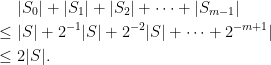
Theorem 1 Let x₀, x₁, …, x_n be a distinct sequence of points of the field F for n < N. If f is a polynomial of degree less than N chosen uniformly at random, then the values

are independent and uniformly distributed on F.

Theorem 1 is straightforward to prove. Consider the number of polynomials of degree less than N and taking values y_i at points x_i. If f₁ is any one such polynomial, then any other one can be written as

where g is a polynomial of degree less than N and vanishing at the points x_i. Since the number of choices for g does not depend on the values y_i, every possible sequence of values has the same probability of occuring.

These considerations show that it is impossible to test whether Bob’s committed function is a low degree polynomial by sampling it at N or fewer points. All is not lost, but it does show that we need Bob to provide more information than just the values of f at Alice’s chosen points.

---

Divide and Conquer

A common algorithmic technique is divide-and-conquer. This breaks a complex problem down into two or more smaller problems. By iterating the procedure, it is eventually broken down into a number of simple calculations, giving an efficient overall approach to the original problem. This is used, for example, by fast Fourier transforms (FFT) which reduce the complexity of computing a discrete Fourier transform from O(N²) to O(NlogN), a significant improvement.

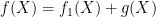
We do something similar. The polynomial f of degree less than N given by (1), can be broken down into two polynomials of degree less than N/2. For example, choosing a positive integer M < N, f can be broken up as

(3)

where u and v polynomials

of degrees less than M and N – N respectively. Choosing M equal to N/2 rounded up to the nearest integer, both u and v have degree less than N/2. Alice can concentrate on showing that they indeed have degree less than N/2, and then that f is equal to u + Xv.

There are many ways of breaking f into lower degree polynomials besides (3). We can, alternatively, split it into odd and even powers of X,

(4)

where u and v are given by

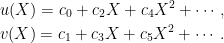Again, the degrees of u and v are both less than N/2. Decomposing f using (4) has several advantages over alternatives such as (3). For one thing, we can express u and v without explicit reference to the polynomial coefficients,

(5)

These identities require dividing by 2, so is only possible in fields where this can be done. The field F of size p^r has characteristic p, meaning that we can divide by any integer which is not a multiple of p. Hence, (5) can be applied so long as F is not a binary field, of size 2^r. For now, we suppose that this is the case, so that (5) applies, and will deal with the characteristic 2 case in a moment. So long as for each x in the domain S, –x is also in the domain, then Alice can use (5) to compute u and v herself.

Another advantage of using (5) is that u and v are not defined on the domain S but, rather, on

If, again, we suppose that –x is in the domain S whenever x is, then the squaring map is 2-to-1 implying that S₁ has half the size of S. This reduces the complexity of the algorithm.

So far, we have reduced the problem of showing that a function has degree less than N, to showing that two separate functions have degree less than N/2. You may well ask, so what? Is it really any simpler than where we started? This is where the next trick comes in. We can combine u and v by taking a random linear combination, and it is sufficient to show that this single function has degree less than N/2.

For a uniformly random field value α, if u + αv has degree less than some value N, then so do both of u and v.

While this statement is not exactly true, it has negligible probability of giving an incorrect result. This is because, if the degrees of u and v were not both within the stated bound, then there would be at most a single field value α for which the degree of u + αv satisfies the bound. This has a probability 1/q of happening, which is negligible so long as the field F is sufficiently large. More precisely, we need to know that if u and v are not both close to a low degree polynomial, then neither is u + αv. This is because Alice does not check the identities at every point of the domain but, rather, only at a random sample, allowing her to check closeness in the relative Hamming metric instead of exact identity. For more details on such estimates, see the 2017 paper by Eli Ben-Sasson, Iddo Bentov, Ynon Horesh, and Michael Riabzev, specifically lemmas 4.3 and 4.4. For now, we note that it is sufficient to prove that u + αv has sufficiently low degree.

We reduced the problem of showing that a function f defined on S has degree bounded by N to showing that the function f₁ = u + αv defined on S₁ has degree bounded by N/2. This method of breaking the problem into multiple smaller problems, which are combined into a single smaller problem, is known as split-and-fold. We can iterate this procedure until it reaches the point that we just need so show that a function f_n is constant on its domain S_n, as shown in figure 3 below.

The algorithm starts with the commit phase. Initially, Bob commits to a function f on domain S. Writing f₀ = f and S₀ = S, the following steps are performed in order i = 0, 1, 2, ….

• Alice selects a random field element α_i and sends to Bob.
• Bob commits to a function f_i + 1 on the domain S_i + 1 = {x²: x ∈ S_i}.

This continues until Bob declares that f_m is equal to a constant value c. Then, in the query phase, Alice does the following for each 0 ≤ i < m.

• Request the values of f_i(x) and f_i(-x) for a randomly chosen set of points x in the domain S_i, and computes the values,
  

  (6)

• Requests the value of f_i + 1(x²) for the selected x-values and verifies that they satisfy
  

  (7)

This is the complete algorithm and, if Alice successfully verifies (7) for all of the points for each i, she declares that f is a low degree polynomial. A few points are in order though. If preferred, equations (6) and (7) can be combined, so that Alice needs to check,

For the special value i = m – 1, she does not need to sample f_i since she can just use the constant value c. The procedure just described is assuming that –x is in the domain S_i whenever x is. Since S_i consists of 2ⁱ th powers of S, this requires S to be closed under multiplying by 2ⁱ th roots of -1. Taking i = m – 1, this means that it is closed under multiplying by 2^m th roots of unity. In particular, the field F of size q must contain all such roots of unity or, equivalently, q – 1 must be a multiple of 2^m. This is not absolutely necessary, since Alice could instead ask Bob to commit to the functions u_i and v_i, and verify that they satisfy

(8)

instead of computing them herself using (6). For efficiency though, it is preferable if F contains 2^m th roots of unity and the procedure above can be used.

Let us also consider the degrees of f_i. By construction, f_m is constant, so has degree less than 1. If f_i + 1 has degree less than a value L and (7) is satisfied on the domain, then u_i and v_i also have degree less than L. So, (8) shows that f_i has degree less than 2L. Hence, f_m - 1 has degree less than 2, f_m - 2 has degree less than 4, and so on, until we get to f = f₀ which as degree less than 2^m. This is exactly as desired in the case when N is a power of 2 and, even if it isn’t, it is usually sufficient to bound the degree by such a power. Alternatively, it is possible to modify the procedure slightly to handle non powers of 2, and I describe one method of doing this at the bottom of the post.

Recall that Alice does not verify (7) at every point of the domain but, instead, at some random sample of n points. This means that she does not really verify that f has degree bounded by N. Suppose we want to be sure that it is within a tolerance ε of such a polynomial in the relative Hamming metric, meaning that it is equal to the polynomial everywhere outside of a proportion ε of the domain. Then, n should be chosen large enough that the probability bound (1 - ε)ⁿ is negligible.

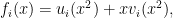
Finally, we can look at the complexity of the algorithm, for a fixed field F and tolerance ε. Since Bob has to commit to a polynomial on each of the domains S_i of size 2^–i|S|, this amounts to committing to a total number of evaluations,

This is only linear in the size of the original domain, so is quite efficient. Alice just requires sampling the functions at a fixed number 2n points of each of the domains S_i, so her work is bounded by 2nm, which is of the order O(logN) so, again, is quite efficient and, in particular, is orders of magnitude lower than the original calculation performed by Bob.

The outline of the FRI algorithm above makes use of the squaring map X² to break the problem into two simpler ones. More general polynomial maps can be used in place of X², as we will see shortly. I only consider quadratic maps in this post, which halves the degree of f at each step. It is possible, though, to use maps of any degree d instead, which reduces the degree of f by a factor of d, although this requires splitting it into d terms instead of 2 at each step.

---

Binary Fields

The algorithm above, based on squaring the elements of the domain, has some issues when the field F is binary of size 2^r. This is because it has characteristic 2, meaning that adding an element of the field to itself (i.e., multiply by 2) always gives zero. Hence, it is not possible to divide by 2, and Alice cannot apply (6) to compute the values of u_i and v_i. In addition, the fact that –x is equal to x everywhere means that the squaring map X² is one-to-one rather than two-to-one. Hence, the domains S_i would all be the same size as S, increasing the complexity.

The method can be rescued for binary fields by using maps

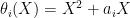in place of just squaring, where a_i is a nonzero field element chosen such that S_i is closed under adding a_i.

As above, the polynomial f_i of degree less than M can be broken down as

(9)

where u_i and v_i are polynomials of degree less than M/2. It can be seen that, in characteristic 2, θ_i(x + a_i) = θ_i(x) for all points in the domain, so θ_i is two-to-one. Alice can solve (9) at any point x by,

(10)

We can ensure that there exist elements a_i with the required property by choosing the initial domain S to be an additive subspace of the field (i.e., closed under addition). Then, the same will be true of each of the domains S_i, and a_i can be taken as any nonzero element of this. The algorithm is then the same as in the previous section, with the modifications described here.

---

Application to STARKS

Recall from the earlier post, that if Bob performs a calculation consisting of N steps, then the execution trace is represented by polynomials of degree less than N. Alice asks for the values of these polynomials, at random points and checks that they satisfy certain identities which encode the calculation transition function as well as the initial and final states. This requires knowing that the values really do come from polynomials, in order to extrapolate the identities from the random sample chosen by Alice to the entire domain. Suppose that they are defined on a domain S in the field F, and Alice compares two polynomials of degree less than ρ|S|. If both sides of the identity are indeed equal, then she correctly verifies this. If they are different, then the probability of them being the same at a random point is bounded by ρ. By sampling at n random points, the probability of incorrectly verifying the identity can be reduced to ρⁿ. So, to ensure that they are indeed polynomials, Alice can use an FRI algorithm as described above to bound their degree, and then verify the polynomial identities. She is, therefore, able to verify Bob’s calculation while keeping the probability of giving an incorrect positive verification below any threshold value.

There are, however, some remaining issues to consider. Even if the polynomials themselves all have degree bounded by the computation length N, the identities involve multiplying them together, increasing the degree and decreasing efficiency. Furthermore, we can remove some of the steps of the algorithm. As an example, let us consider a sequence of N Boolean values represented by a polynomial f of degree less than N. The fact that it only takes values 0 and 1 in the calculation is represented by the identity

(11)

where Z is a pre-specified polynomial of degree N vanishing at all field points used to represent the execution trace. The term p is referred to as the quotient polynomial, and also has degree bounded by N. I will suppose that, for the purposes of this discussion, Alice is able to compute Z herself. Then, according the outlined argument above, she could separately verify that f and p have degree bounded by N and then verify that (11) holds at random points. Note, however, that the both sides of (11) can have degree anything up to 2N – 2. In fact, once it is verified that f is a low degree polynomial, it is not necessary for Alice to separately check that p is low degree and that (11) holds. As p is not used anywhere else, instead of asking Bob to commit to it, she can define p by

(12)

So, all that remains is to check that this is indeed a low degree polynomial using the FRI algorithm without separately checking (11).

This procedure can be made slightly more efficient still. Recall that, for the polynomials interpolating the execution trace, there are two kinds of polynomial relations to be checked. First, there are those which enforce properties of the entire execution trace, such as enforcing the transition function and any further fixed properties, such as representing a Boolean variable. Second, there are those enforcing the initial and final condition, which are of the form

(13)

where Z₀ is a low degree polynomial vanishing only at the initial and final times, Z₀ = (X - x₀)(X - x_N-1), and u is a similarly low degree polynomial giving the correct initial and final values. Using the ideas outlined above, this would be rearranged as

and we show that the quotient polynomial q is low degree. Alternatively, the procedure can be made a bit more efficient by using (13) to eliminate f entirely. Instead, the prover Bob just provides his commitment to q, which needs to be shown to be of low degree. Equation (13) is used to replace occurrences of f in expressions such as (12) with q.

As a final point, note that it will generally be required for Alice to verify that several polynomials all have low degree. This could be done by separately applying the FRI algorithm to each of them. Alternatively, they can be combined in much the same way as described for the ‘split-and-fold’ method above. If Alice wants to show that polynomials f₀, f₁, …, f_n all have low degree, then she can form a random linear combination,

Here, α₁, …, α_n are independent uniformly random points of the field. It is only necessary to show that this combination g is low degree to imply, up to a negligible probability, that each of the terms f_i are low degree.

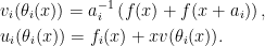
Here, ‘low degree’ means that it is a polynomial of degree less than that ensured by the FRI algorithm which, as described above, will generally be a power of two, 2^m. This can be generalized to prove that each f_i has degree less than specified value N_i ≤ 2^m. We just note that this is equivalent to f_i and X^2m - N_if_i both being polynomials of degree less than 2^m. So, using the same ideas as above, we just need to choose a random field value β and apply the FRI algorithm to

Combining these ideas, in order to show that each f_i has degree less than N_i, we pick random field values α_i, β_i and apply the FRI algorithm once to the combination

Hence, no matter how many polynomials are used to represent Bob’s calculation, only a single FRI proof is required in a STARK algorithm. We could even combine multiple STARK proofs, which would give the significant efficiency of being able to combine their FRI proofs into one.